The Pacific War Online Encyclopedia
|
| Previous: Finschhafen | Table of Contents | Next: Firefly, British Carrier Fighter-Bomber |
U.S. Navy. Via
ibiblio.org.
Click to elnarge
Guns can destroy only what they can hit. This was a difficult problem for long-range gunnery against moving ships, which required the gun to place the shell where the ship would be when the shell arrived. At maximum battle range of about 28,000 yards (25,600m), a 16" (406mm) shell could take 40 seconds to reach the target, and a target steaming at 25 knots would have moved 560 yards (510m) while the shell was in flight. This was nearly twice the length of an Iowa-class battleship. Long-range fire control proved more difficult for naval engineers to perfect than the construction of guns capable of throwing shells to great distances. However, fire control advanced rapidly during the first part of the 20th century, and by 1939 fire control was one of the most sophisticated of naval technologies. The major naval powers closely guarded their fire control secrets, yet most fire control technology was derived from the British, and no one power had a decided advantage until the introduction of radar. Radar revolutionized fire control during the Pacific War and strongly favored the Allies.
Much of the impetus for developing long-range antiship gunnery came from the torpedo. Torpedoes could inflict massive damage, and it was felt that gunnery could compete with torpedoes only if guns could hit their targets from outside of torpedo range. The race between long-range gunnery and torpedoes reached its end point with the U.S. 16"/50 gun and the "Long Lance" torpedo; the 16" gun could theoretically hit a target at 42,000 yards (38,000 m) under perfect conditions, while the Long Lance had a maximum range of 48,000 yards (44,000 m) at its slowest speed setting (though this was rarely used.)
Small guns with limited range used simple telescopic sights. The gunner made his best guess at the range, set the elevation accordingly, put his cross hairs on the target, and kept them centered as his own ship rolled (continuous aim). Opinions differed on which was the best point in the ship's roll to fire, but most gunners tried to fire at the beginning or end of the roll, when the ship was momentarily stationary. At such close ranges, shell trajectories were relatively flat, and range could be adjusted by eye. This procedure was completely inadequate for long-range fire, whose accuracy depended on a correct handling of target tracking and position prediction, interior and exterior ballistics, computation, and correction.
Interior and Exterior Ballistics. Interior
ballistics is concerned with the physical processes that determine
the velocity with which the projectile leaves the barrel. Exterior
ballistics is concerned with the behavior of the projectile after
it leaves the barrel. In principle, the latter is a
straightforward question of physics, involving gravity, the
Coriolis correction for the earth's rotation, and the atmospheric
drag force (adjusted for wind) on the projectile. In practice, the
ballistics were tested against each pairing of gun model and shell
type on the proving ground, where the results of carefully
controlled firings at different compass bearings and elevations,
for powder at various temperatures, and for guns in various states
of wear could be painstakingly measured and tabulated under
varying weather conditions. The more exhaustive the testing, the
more accurate the results, but also the more expensive the testing
program.
|
U.S. Navy. Via Friedman (2008) |
U.S. Navy. Via Friedman (2008) |
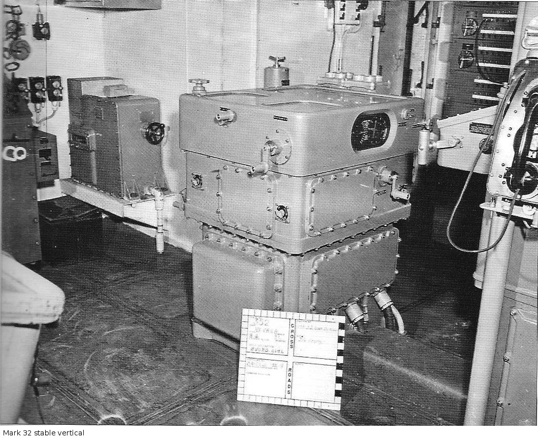
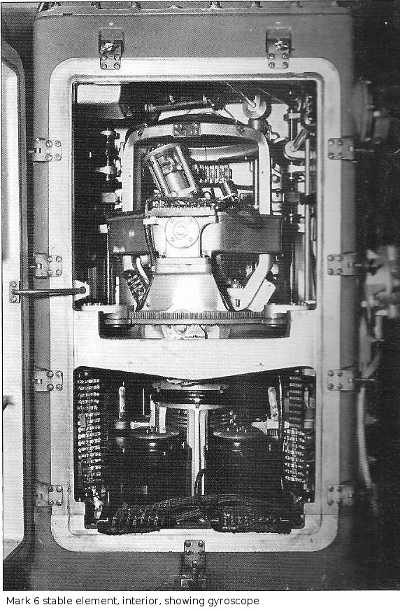
Deck Motion. Deck motion due to ship roll
(rocking from side to side), pitch (rocking from bow to stern),
and yaw (rocking around the vertical axis of the ship) from wind
and waves were also well understood, and methods for compensating
for deck motion began to be developed as early as 1898. Hydraulic
machinery made it possible to continuously aim heavy guns, and
gyroscopes helped automate the process. The Mark 32 director
(shown above, left) provided a stable vertical for compensating
for ship motion. The view of an interior of a Mark 6 (above,
right) shows the gyroscope providing a stable element.
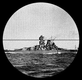
Determining Bearing and Range. Obtaining an
accurate bearing was a straightforward matter of providing the
fire control party with telescopic sights, except under conditions
of poor visibility, when fire control radar became increasingly
important. Range was typically provided by optical range finders
early in the war and by fire control radar as this became
available.
Optical range finders were either coincidence or stereoscopic range finders. Both used large telescopes or prisms at opposite ends of a long crossbar. In a coincidence range finder, the images from the two prisms were combined in a single eyepiece, but matched exactly only when the observer adjusted the range finder to the exact range to target.
Coincidence range finders came in two variants. The older versions showed the image from one telescope in the upper half of the field of view and from the other telescope in the lower half. The observer selected sharp vertical features in the images, such as masts, and adjusted the range until the features were continuous across the boundary between images:
Later, rangefinders were developed that inverted the lower image, which was thought to make finding the coincidence easier:
Stereoscopic rangefinders worked like a pair of binoculars, with two eyepieces. The observer's eyes and brain brought the images into coincidence, and range was obtained using a set of marks in each eyepiece that were adjusted until they appeared to be at exactly the same range as the target. The U.S. Navy concluded in 1941 that there was little to choose between the two kinds of range finders.
Rangefinders were best located high in the ship, but the
Americans also installed rangefinders in main gun turrets, where
they benefited from the protection of the heavy turret armor.
These were known as "battle rangefinders".
Fire control radar obtained the range by measuring the time for a radar pulse to reach the target, be reflected, and return to the radar set. Radar was far more reliable under conditions of poor visibility than optical range finding, and it could not be foiled by dazzle camouflage. A skilled radar operator could obtain an accurate range to target almost at once, whereas optical range finding required repeated observations to build up an accurate range estimate.
Enemy Course and Speed. In addition to knowing
the bearing and range, it was necessary to know the rate of
change of these quantities, in order to calculate where the
target would be when the shells arrived and aim the guns
accordingly. This could be computed from one's own course and
speed and the enemy course and speed using a simple mechanical
calculator, such as the British Dumaresq or the American Rate
Projector. One's own course and speed were of course known,
but the enemy course and speed had to be measured or estimated.
The initial estimate of enemy course could be obtained, if one
knew the length of the enemy ship, by measuring its angular length
using an inclinometer and comparing this with the range. A ship
approaching on a rapidly converging course is significantly
foreshortened. A trained
observer could also estimate course from the apparent angle on the
bow, but this was uncertain and was resorted to only when the
enemy ship's length was uncertain. Speed could likewise be
estimated by a trained observer from the bow wave.
Spotting aircraft were particularly valued, not only because they could see further, but because an observer in an aircraft high above the water could often make a significantly better initial estimate of enemy course and speed than a shipbound observer.
U.S. Navy. Via
Friedman (2008)
Prediction. Once the target bearing, range, course, and speed were known, one could calculate the aiming point. This was not an entirely straightforward calculation, because the bearing and range rates were continuously changing even when both one's own ship and the target were on steady courses. The computations were done using mechanical computers into which the data could be fed. The simpler fire control computers still in use at the time of the Pacific War were analytic computers, which simply took the input data and returned the current solution. These were used on smaller warships where there was no room for more sophisticated fire control computers and their operators.
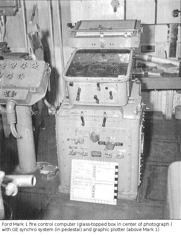
Larger warships used synthetic fire control computers,
such as the Ford Mark 1 shown above. Synthetic fire control
computers not only returned the firing solution for the current
estimates of the targeting data; they also integrated the rate
equations to predict future range and bearing on the target. The
subsequent discrepancy between the computer solution and the
predicted solution could be fed back into the computer, greatly
improving the fire control solution.
The Ford fire control computer was first developed in
1917 and the Mark 1 Mod 3 continued in use on older battleships
through the Pacific War. It was eventually replaced with the Mark
8, beginning with the reconstruction of the New Mexicos and
on new cruisers from the New Orleans
class on. Smaller warships used the Ford Mark 2, or "Baby Ford",
which was a compact, simplified version that did not compute
bearings and could not benefit from feedback.
The British equipped their warships with various models
of the Admiralty Fire-Control Table (AFCT), which could return a
firing range within five seconds. The Mark 6 was used on the most
modern cruisers, while rebuilt battleships used the Mark 7 and
newly constructed battleships used the Mark 9. The Mark 10, which
was the first fire control computer to correct for enemy changes
in course, was not ready in time for the war. Destroyers used a
simplified fire control computer called the Admiralty Fire-Control
Clock (AFCC) that lacked plotters.
The Japanese relied on the Type 92 Computer and Sokutekiban (or, on the Yamatos, the Type 98 Director, Computer, and Sokutekiban). The Japanese word Sokutekiban has no good English equivalent, but denotes a device for computing target course and speed. The Japanese fire control equipment was excessively heavy and manpower intensive, requiring all inputs to be entered manually. However, Japanese optics were excellent, their range tables sophisticated, and their crews well-trained. The Japanese determination to match Western fire control using heavy, manpower-intensive fire control technology explains the tall, heavy masts seen on many Japanese warships, which were known to the Allies as "pagoda masts."
Correction. There was always some systematic
error in an initial fire control solution, no matter how good the
data fed to the fire control computer, due to variable atmospheric
conditions, gun wear, slight miscalibration of the equipment, or
other subtle causes. Thus, the first salvo fired at the target was
very likely to miss. Based on which direction the shells missed,
the fire control solution was adjusted to bring the next salvo
closer to the target. This was known as searching the target area.
Shells that actually hit were very difficult to observe,
and those that went over the target were also not easily observed
except by spotting aircraft. As a result, the seemingly sensible
approach of firing one or two shells and saving the full salvos
until the fire control solution was adjusted onto the target was
not actually very practical. However, elaborate schemes were
worked out to make the most of a single salvo or a set of salvos
from several ships concentrating their fire on a single target.
The British favored the ladder system, in which several salvos
were fired at slightly different ranges to quickly determine the
correct range.The Americans, who anticipated fighting in more
placid seas, developed instruments to calculate the range error by
measuring the angle between the target waterline and the shell
splash. However, by the time of the Pacific War, the British had
worked out four standard salvo groups. These were a deflection
group to find or regain bearing, a ladder group to find or regain
range, a zigzag group to rapidly refine a good target solution,
and a rapid group to exploit a refined fire solution. The first
three groups used two or three salvos, with the third salvo
canceled if the first two were far off target, while the rapid
group consisted of four salvos.
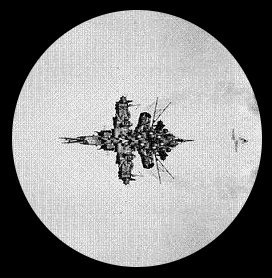
Radar transformed spotting, since shell splashes proved
to be easily visible on radar and gave a very accurate correction.
Indeed, the success of fire-control radar meant that Allied
warships had landed their spotting aircraft by 1943, since these
could not operate at night and were a severe fire hazard if their
ships were hit by enemy fire.
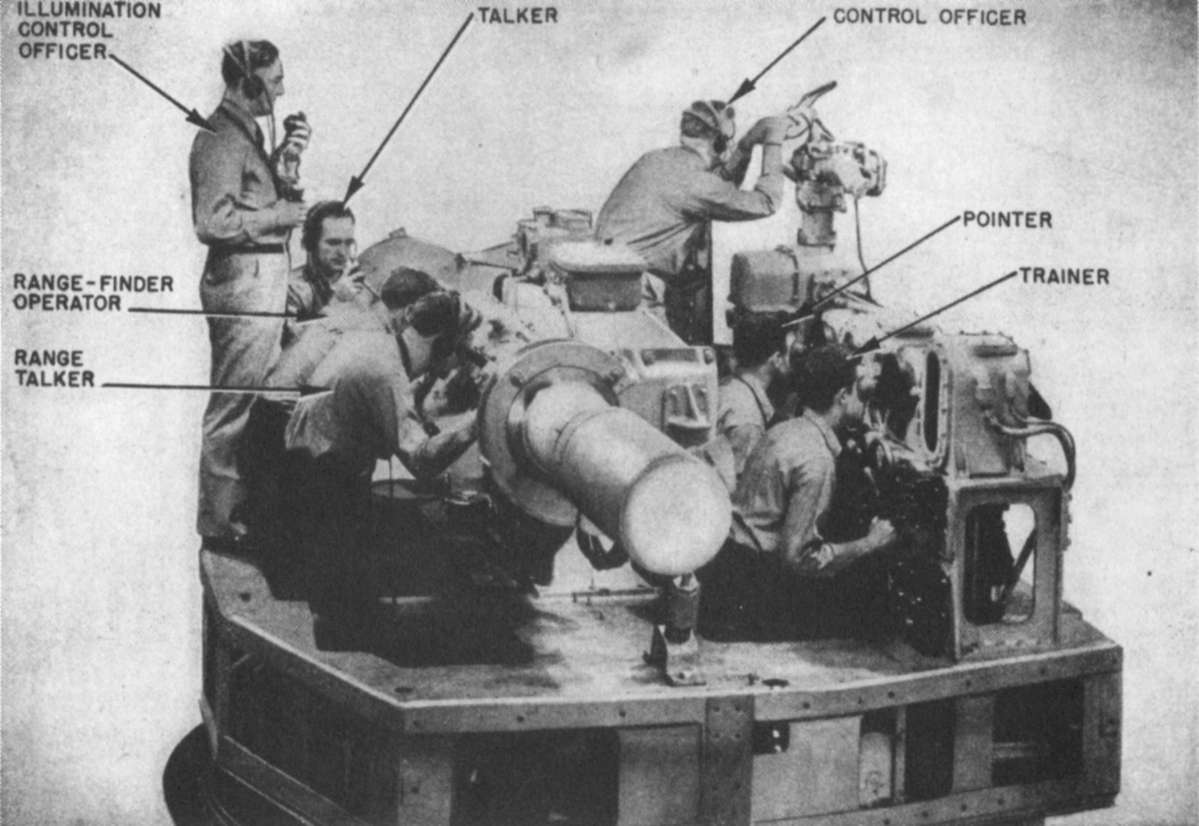
Salvo fire required that all the guns firing the salvo be controlled from a central location, rather than from the individual guns. This was done from a director, which was an observation point high in the ship from which all the guns in a salvo could be fired electrically using a master switch. It was only natural that the director should also include the various sighting telescopes, rangefinders, and other instruments used to collect data for fire control. The British attempted to include early fire control computers in the director itself, and this continued to be the practice with directors for smaller warships, such as the U.S. Mark 18 8" cruiser gun director, or for secondary batteries on larger warships. However, the fire control computers and their operators for the main batteries of cruisers and battleships were too bulky to be included in the director, and they were kept in a separate plotting room within the armored citadel of the ship. This also protected the fire control computers from enemy fire. The directors themselves could not be heavily protected, since they were high in the ship and needed a clear view of the outside world, but large warships were equipped with more than one director so that, if one was destroyed by enemy fire, another could take over.
Concentration of fire from more than one warship was a problem. Several ships firing on a single target would confuse each other's salvos and spoil their fire control solutions. The solution was to have ships fire in succession, so that they could distinguish their own salvos. Once the range was found, the ships would shift to rapid fire. In addition, following the First World War, many navies installed large range clocks on their masts, which communicated range information from ship to ship.
In order to filter out random errors, the measured ranges and bearings were plotted against time on a roll of graph paper. Such tracking boards were often built into the fire control computer itself. The human plotter could look at a scattering of range estimates and extrapolate a curve through the measurements, something that was beyond the capability of simple mechanical computers. A pointer could typically be laid along the extrapolated curve and its position and direction was automatically fed into the computer.
The greatest limitation of fire control computers of the
Pacific War was that they assumed the target was on a steady
course. They could not easily accommodate changes in course by the
target. However, the most sophisticated fire control systems could
take into account one's own changes in course. This sometimes led
to situations like that at the Battle of the
Komandorski Islands, in which both sides had fire control
that allowed their own ships to maneuver freely but which could
not take into account the enemy's maneuvering. The battle was
notable for a very poor hit rate by both sides even though it took
place in daylight at the anticipated battle ranges. With the
introduction of Mark 3
radar, the Americans all but abandoned spotting in favor of
rocking salvos back and forth across the measured target range.
Elements of a Fire Control System. From the discussion so far, we see that a fire control system required sensors (telescopes, rangefinders, inclinometers, or radar) to collect data on the target; gyroscopes to account for the ship's own motion; computers to calculate the firing coordinates; and mechanisms for transmitting the data back and forth between these elements.
The simplest means of communication was to communicate by voice over voice pipes or telephones, but this was highly unreliable in the din of battle. More reliable was cyclometers (resembling the odometer in an automobile) that could be turned to the correct number using stepper motors. However, this proved too slow and clumsy. "Follow the pointer" systems moved a pointer to the desired position on a dial (such as a range dial on a gun) which was then matched by the gunner. This proved highly effective, but by the time of the Pacific War, "follow the pointer" had been superseded by servos that allowed the gun to be aimed directly by the fire control computer. Stepper motors continued to be the basic transmitting mechanism, having become very fast and highly reliable.
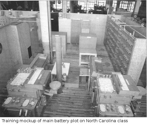
Thus a battleship fire control system consisted of director stations with all the instrumentation required to track the target; one or more plotting rooms within the armored citadel that contained the fire control computers; and transmission lines between the directors, the fire control computer, and the guns. This formed a data network for the ship. As radar drove the development of Combat Information Centers, these were also wired into the data network. Most of the more modern cruisers also had plotting rooms, and even destroyers began to acquire CICs by the end of the war. The chief distinction between a plotting room and a Combat Information Center was that the former was dedicated exclusively to determining the fire control solutions for one's own ship, while the CIC was concerned with keeping track of the overall tactical situation by plotting all known friendly and enemy units.
U.S. gunnery fire control was second to none at the start of the Pacific War, having undergone what Evans and Peattie (1997) have described as "a second gunnery revolution" in the late 1930s. Among the most important American advantages was the high quality of the gyroscopes used to automatically correct for deck motion and accurate, high power, remote controlled servomechanisms (synchros) for aiming the guns. The U.S. Navy defined four range bands: extreme range beyond 27,000 yards (24,700m), long range from 21,000 yards (19,200m) to 27,000 yards; moderate range from 17,000 yards (15,540m) to 21,000 yards; and close range below 17,000 yards. The Tennessee and Colorado classes were thought to be superior at extreme range and the other U.S. battleships at their best at moderate range. The Navy assumed that air spotting would be required beyond 28,000 yards (25,600m) and that gunfire without air spotting would lose half its effectiveness beyond 22,000 yards (20,100m).
|
Training
mockup of main battery plot of North Carolina. U.S.
Navy. Via Friedman (2008). Click to enlarge. |
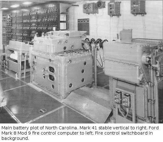
Main battery plot of North Carolina. U.S.
Navy. Via Friedman (2008). Click to enlarge |
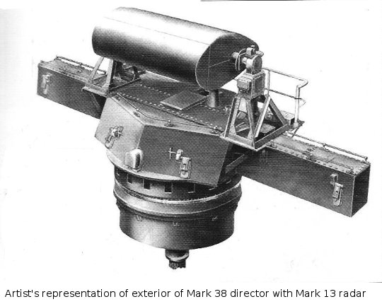
Mark 38 director. U.S. Navy. Via Friedman (2008) |
The Bureau-Sperry fire control system in U.S.
battleships typically consisted of two separate Ford Mark 1
computers in their plotting room (allowing two targets to be
tracked simultaneously) and three directors, two in the mastheads
and one in the conning tower, plus additional directors in the
superfiring turrets of newer battleships. These were connected by
stepper repeaters. The systems were upgraded periodically,
particularly after the advent of radar, and the modern ships of
the North
Carolina class onwards had the Mark 38 director shown
above. This was originally equipped with a 26.5' (8.08 m)
rangefinder, but this was quickly superseded by fire control
radar. It could train at 10 degrees per second and weighed 40,000
lbs (18,100 kg) in most models or 50,000 lbs (22,700 kg) in later
models. The secondary dual-purpose battery of the modern
battleships used the Mark 37 director shown in cutaway at the top
of this article.
The British and, especially, the Japanese trailed behind the Americans. Though Japanese optics were excellent and their crews well-trained, in the only long-range daylight gunnery duel of the war (Komandorski Islands), the Japanese came out second best.
Both Washington
at the Naval Battle of Guadalcanal and West Virginia at
Surigao Strait straddled their
targets with their first salvos. However, it was typical for only
a modest percentage of shells even from accurate salvos to
actually hit the target. Washington hit Kirishima off
Guadalcanal with just 20 out of 75 main battery shells fired, a
rate of 27%, in spite of radar fire control. The Japanese likewise
claimed that Nagato
achieved 12% hits at 35,000 yards (32,000 meters) in a prewar
exercise under ideal daylight conditions using spotter
aircraft. During the Battle of the Java Sea, the Japanese
cruisers fired 1271 shells at the Allied cruisers at ranges of
21,900 to 27,300 yards (20,000 to 25,000 meters) and scored just
five hits, four of which were duds. During the night action at Empress Augusta Bay,
the American force fired 4591 6" shells and scored perhaps 20
hits. This hit probability of 0.4% was not unusual for the Solomons campaign,
where most of the surface actions of the war were fought.
In most respects, torpedo fire control was simpler than gunnery fire control. A salvo of shells could only hit a target located in a relatively small patch of ocean on which the shells fell. A torpedo could hit a target anywhere along a path that could be miles long. In the language of fire control, a torpedo had a much larger danger space than a salvo of shells. This, and the massive damage that could be inflicted by a torpedo's large explosive charge, did much to make up for the fact that the torpedoes usually had to hit with the first salvo.
However, torpedo accuracy had its limitations, and prewar torpedo tactics included the use of "browning shots" aimed against entire enemy formations steaming in line ahead rather than against individual ships. Such tactics were actually employed by the Japanese in the night battles of the South Pacific, where the almost instinctive response of the Japanese when ambushed was to launch shoals of torpedoes in the direction of the enemy. These tactics proved devastating in the earlier battles, and it took the Allies some time to come up with adequate counter tactics.
Initial estimates of the target's range, course, and speed were obtained through the submarine periscope. The periscope operator (who was almost always the submarine commander) estimated range using a stadimeter, which measured apparent angle between waterline and masthead. Assuming the height of the mast was known, the stadimeter immediately gave the range. Thus, ship identification books issued to submariners always listed the masthead height. Speed was then estimated either as the likely cruising speed of the target, possibly modified by the appearance of the bow wave, or by propeller rotation count from the sonar operator. Angle on the bow, which gave course, was estimated by simple observation, a skill which was carefully developed during training.
The fire control computers that equipped the submarines of most
World War II naval powers were simple analytic computers that gave
an instantaneous solution based on the current best estimates of
bearing, range, course, and speed. For example, the obsolescent
submarines of the S-1
and S-42 classes
used a handheld mechanical calculator, the Mark 3 Torpedo Angle
Solver, nicknamed the "banjo" for its shape.
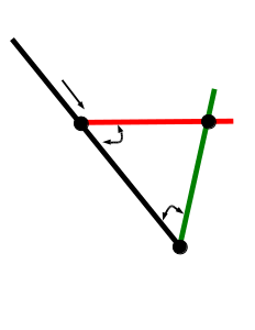
A mechanical torpedo fire control computer consisted of three
basic elements, each consisting of a scaled rod. The first rod (in
red) represented the target's course and speed, with the scale
marked in knots. The second rod (in green) represented the torpedo
course and speed, and likewise was marked in knots. These were
joined to each other and to a third rod (in black) representing
the bearing to target, which was also scaled in knots. These three
elements were joined to form a triangle, known as the fire
solution triangle. The torpedo rod and bearing rod were joined by
a simple pivot, while the torpedo rod and target rod were joined
by a pivot that could be slid along each rod and screwed down at
the appropriate speed marking. A third pivot joined the base of
the target rod to the bearing rod, and could be slid along the
bearing rod. The diagram below shows the fire control triangle,
with arrows to indicate the way in which the fire control officer
could move the elements once the target and torpedo speeds were
set.
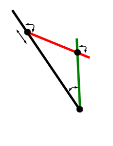
Finding the fire control solution was now a simple matter of
sliding the base of the target rod (red) along the bearing rod
(black) until the angle between the target rod and bearing rod
matched the estimated target course relative to the target
bearing. The angle between the bearing rod and the torpedo rod
(green) gave the desired torpedo bearing relative to the target
bearing.
In effect, the mechanical computer allowed the fire control officer to construct a small scale model of the fire solution. The earliest fire control computers were no more complicated than this. Later computers placed the entire fire control triangle on a protractor, to simplify converting bearings relative to the target to bearings relative to the firing ship.
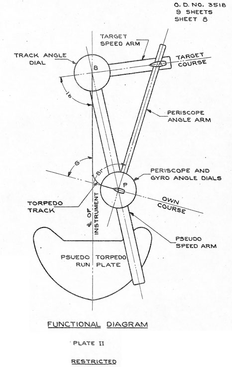
With the introduction of torpedoes that could be set to turn to a new bearing after being launch, an additional element, which the Americans called the pseudo torpedo run plate, was required to take into account the fact that the torpedo did not turn onto its final bearing all at once. This required more fiddling with the "banjo" to get a good solution.
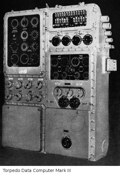
The TDC (Torpedo Data Computer) carried by the more modern
American submarines was a
sophisticated synthetic fire control computer. Though the TDC
automatically worked the basic four elements to obtain the firing
solution, its more important contribution was to allow the fire
control officer to build up an accurate estimate of enemy course
and speed. While submariners of other nations could, and did,
check their estimate of the target speed by observing how quickly
the target moved across the periscope field, the TDC calculated a
continuous prediction of target range and bearing which could be
matched against further observations to correct the range and
bearing rate.
The usual defense against submarine torpedo attack was for ships
to follow a zigzag course, periodically switching their heading
from side to side of the baseline course.Such periodic course
changes could spoil the fire control solution of any submarine
lying in wait. However, a sufficiently skilled and patient
submarine commander could work out the zigzag pattern of the
target he was pursuing and quickly develop a fire control solution
after a favorable zigzag (which was usually a zigzag towards his
own position.)
Heavy antiaircraft guns had complicated directors,
often separate from the gun itself, that resembled those for
surface fire control. These calculated the proper lead so that the
shell and its target would arrive at the same point in space at
the same moment in time. The director also controlled a fuse
setter for timed shells that set the shell to detonate just before
the estimated moment of closest approach. Both lead calculation
and fuse setting required an accurate estimate of the range to the
target, which was originally provided by an optical range finder.
These were of limited accuracy compared to radar range finders.
Naval antiaircraft directors had the additional challenge of
compensating for the rolling of the ship, which was accomplished
using gyro stabilization, as with the main battery.
Light antiaircraft guns were originally equipped
with very simple sights, and the gunner determined the correct
lead on the target by observing his tracer rounds and adjusting
his aim accordingly. Fire control was rapidly improved with
gyroscopic sights, where the gunner simply followed the target
with his gun sight. The gyros automatically measured the motion of
the gun sight and added the correct lead based on the range to the
target. By the end of the war, U.S. light antiaircraft was being
equipped with radar directors that had full blind-fire capability.
The U.S. Navy fielded the best heavy antiaircraft
director of the war, the Mark 37, which was originally equipped
with an optical range finder but was repeatedly upgraded with
improved radar range finders. The Mark 14 and Mark 15 gyrosights
were used on the 20mm Oerlikon and were also incorporated in the
Mark 51 and Mark 52 directors for the 40mm Bofors. The Mark 51 was
often cross-connected to a warship's 5"/38 guns to give them some
usefulness against targets at short range.
Japanese antiaircraft fire control was poor throughout the war. The Japanese started the war with the Type 94 director for heavy antiaircraft fire, which proved much too slow. After the disaster at Midway the Japanese Navy rushed development of the Type 3 director, but the prototype was never completed. The Type 95 director for light antiaircraft was available only for triple 25mm mounts, all others using open ring sights. The low quality of Japanese antiaircraft fire control was manifest at the Battle of the Sibuyan Sea, when only 18 Allied aircraft were shot down out of hundreds attacking a Japanese force equipped with hundreds of antiaircraft barrels.
The key element for fire control against a submerged submarine was a British invention called the chemical recorder. This was a rotating drum of chemically treated paper with a stylus, resembling nothing so much as a modern seismograph. The rotations of the drum were synchronized with the pings from an active sonar set, and the stylus was connected to the receiver and twitched when an echo was received. The result was a series of marks on the paper that allowed the operator to directly read off the range rate and estimate the change of range rate. This allowed accurate timing of depth charge drops.
Attempts were made in 1939 to use the range recorder to
automatically fire an ahead-thrown weapon, but this was a single
light charge that proved unsuccessful. However, the idea was
applied much later to Hedgehog.
During the war, a second recorder was added to track the bearing
rate, creating a fire control system that began to resemble a
synthetic surface gunnery fire control system.
References
FleetSubmarine.com
(2002; accessed 2013-9-28)
NAVPERS
16116A (1946-3; accesssed 2013-7-15)
NAVPERS 91900 (1953; accessed 2012-4-30)
"Torpedo Data Computer," BuOrd 1056 (1944-6; accessed 2013-9-28)
The Pacific War Online Encyclopedia © 2013-2014, 2017 by Kent G. Budge. Index